1. Introduction

The self-organizing map (SOM) has been widely used as a software tool for visualization of high-dimensional data [1]. Important SOM features include information compression while trying to preserve topological and metric relationship of the primary data items. Similar input data should be mapped to the same neuron or in a nearby unit, but this assumption of topological preservation is not true for many mappings involving SOM in dimension reduction [2]. The clus­tering properties of a trained SOM with two-dimensional output grid can be visualized by the U-matrix, which is a neuron’s neighborhood distance based image [3, 4]. With the automation of cluster detection in SOM [2] higher output dimensions can be used in problems involving discovery of classes in multidimensional data.

The lower difference between intrinsic dimensional­ity of the input space (data) and output grid the better topological preservation in Kohonen maps. This paper presents the U-array as an extension of the U-matrix for 3-D SOM output grids. The advantage in working with higher dimensions is the better topological preservation in data analysis. The algorithm uses the watershed transform to perform the SOM segmentation. Markers are found by performing a multi-level scan of connected regions of the U-matrix. Exam­ples of automatic class discovery using U-arrays are also presented.

2. U-array and its segmentation

The U-array is proposed as an extension of the U-matrix for 3-D SOM output grids. The advantage in working with higher dimensions is the better topologi­cal preservation in data analysis. The present paper deals with 3-D output grids. We have the common neu­ron’s neighboring distances of the U-matrix (dx, dy e dxy), and the new distances dz, dxz, dyz e dxyz. Figure 1 shows these distances for a map with size 2´2´2. For easy of visualization only output relations between neurons are presented and only one of each type of distance are shown.

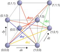
Figure 1 – Distances between neighboring neurons in a map with size 2´2´2

All distances are composed in a similar fashion of the U-matrix, defining a cube with size (2X-1) ´ (2Y-1) ´ (2Z-1) for a map with output grid with size X ´ Y ´ Z. The dxyz distance is a mean of the distances of opposite vertices in the cube, given by

Considering for example the indexes of figure 1,  a  3´3´ 3 U-array is obtained. Agreeing with the U-matrix, the obtention of du values (not shown) can be per­formed by simple interpolation, using mean or median values of neighboring distances.

2.1 Segmentation of the U-array

 The algorithm for segmentation of the U-array uses the watershed transform to detect regions of neurons that belongs to data clusters.

A major steps of the segmentation algo­rithm is the definition of the watershed markers. Let f be the U-array of a trainned map, of size 2N-1 ´ 2M-1 ´ 2K-1, where N ´ M ´ K is the size of the map. Consider [f_min, f_max] = [0, 255] and n_i = 1, i.e., the image f (array) has 256 gray levels. The following steps are performed (algorithm to find watershed markers):

 1.  Filtering: create the image f₁ by removing any pore with area less or equal than three pixels (voxels).

2.  For k = 1 to f_max, where f_max is the highest gray level of the image:

2.1 Create the binary image U₁^k  that corresponds to the conver­sion U₁  to a binary image using as threshold k.

2.2 Obtain N_cr^k, the number of connected regions of U₁^k.

3. Obtain the most persistent value of number of regions h (clusters of neurons) that corresponds to the highest (and significant) plateau in the plot of N_cr^k versus k.

4. Take as image marker the binary image U₁ⁿ, where n is the initial value k of the plateau chosen in the previous step.

 

The basic steps of the U-array segmentation algorithm are:

   1. Obtain the U-array using the trained map;

2. Find the image markers;

3. Impose the new regional minima by modification of image homotopy (or gray-scale geodesic reconstruction);

4. Compute the watershed lines [5];

5. Assign a differ­ent label for each connected volume (clus­ter of neurons) of the U-array [2].

6. Copy the U-array labels to the corresponding neurons in the map.

 

3. Application example: chainlink data set

 The chainlink data set [3] consists of 1000 points in ³-space arranged such that they form the shape of two intertwined three-dimensional rings. The two rings can be thought of as two links of a chain with each one consisting of 500 data objects. This problem illustrates the capabilities of finding the structure of the data even for non-spherical, complex shaped and non-linearly separable clusters.

The SOM grid size for this experiment was 8´8´8 neurons and the number of training epochs (batch algo­rithm) was 200. Figure 2 shows the resulting configura­tion of neurons in the 3-D space after the unsupervised training. Neighborhood in the SOM grid are ex­pressed by the lines connecting the neurons. The correspond­ing U-array is given in figure 3. Figure 4 present the segmented 3-D grid, without link neurons (neurons that do not quantize data items).

 

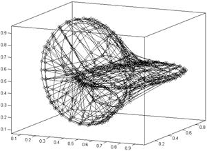
Figure 2: Grid of the map after 200 epochs (batch algorithm).

 

 Figure 3: U-array for SOM presented in figure 3

 

 Figure 4: Labeled 3-D grid after U-array segmentation

 4. Conclusions

 This paper focused the usage of SOM as a clustering tool and some of the additional procedures required to enable a meaningful cluster's interpretation in the trained map. Most of the applications of Kohonen maps use 2-D output grids because a major application is data visualization. With the automation of cluster dis­covery by using algorithms for image and volume seg­mentation [2], as well the use of methods of graph parti­tioning [6], in the context of SOM neural networks, new software tools can be developed for automatic data classification. Further work are needed in order to dis­cover the best output grid for a given data set, and to extend the U-array method for p (p > 3) output dimen­sions.

 

 References

 [1] Oja, E. and Kaski, S. (Eds.). Kohonen Maps, Elsevier, Amsterdam, 1999.

[2] Costa, J.A.F. Automatic classification and data analysis by self-organizing neural networks. Ph.D. Thesis (in Portuguese). State University of Campinas (Unicamp), SP, Brazil, 1999.

[3] Ultsch, A. “Self-Organizing Neural Networks for Visualiza­tion and Classification”. In: O. Opitz et al. (Eds). Information and Classification. Springer, Berlin, pp. 307-313, 1993.

[4] Vesanto, J. and Alhoniemi, E. “Clustering of the Self-Organizing Map”, IEEE Tr. Neural Networks, 11 [3], p 586-602.

[5] Falcão, A.X., Stolfi, J., & Lotufo, R.A. “The Image Forest­ing Transform: Theory, Algorithms and Applications”, IEEE Trans.Pattern Analysis & Machine Intelligence,26[1], pp.19-29.

[6] Costa, J.A.F., and Netto, M.L.A., “Segmentação do SOM Baseada em Particionamento de Grafos”. In: Proc.VI Brazilian Conf. on neural networks, São Paulo, pp. 451-456, 2003.